Understanding embedding models: make an informed choice for your RAG

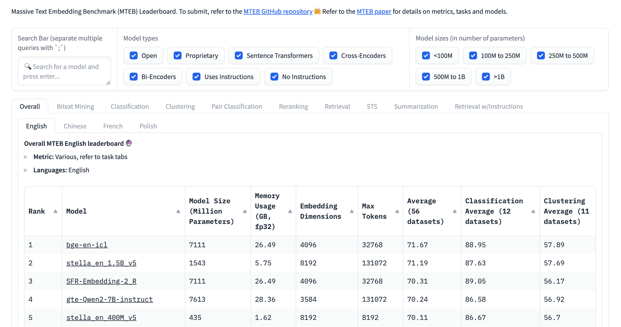
How do you choose a suitable embedding model for your RAG application? A popular starting point for selecting a text embedding model is the Hugging Face MTEB (Massive Text Embedding Benchmark) leaderboard, as shown below:

However, if you’re new to embeddings, this leaderboard with all its various tabs, filters, and metrics, may appear somewhat intimidating. If that’s the case, you're in the right place! This post will help you navigate the embedding models and the leaderboard with ease. You’ll learn: 

• When to use a Bi-Encoder and a Cross-Encoder

• What happens during a Bi-Encoder pre-training

• How embedding models are benchmarked

• How to select a baseline embedding model for your use case

• How to improve upon baseline embeddings

Let’s start by unpacking how we calculate similarity between two pieces of text using encoder transformer models. 

Bi-Encoders vs Cross-Encoders

When it comes to calculating similarity between sentence or document pairs, there are two primary approaches: Bi-Encoder transformer models and Cross-Encoder transformer models. You may have noticed the checkbox filters for both of these in the MTEB leaderboard. The models used to generate vector representations of your data for the RAG’s knowledge base are Bi-Encoders. However, Cross-Encoders also have a role to play in RAG systems, so let's dive into the differences between them.

Bi-Encoders produce a vector representation for a given sentence or document chunk; which is usually a single vector of a fixed dimension. Note that there’s an exception to this - ColBERT, but we won’t be covering it in this blog post. In most cases, whether the input text is a single sentence, such as a user question, or a full paragraph, like a document excerpt, as long as the input fits within the embedding model's maximum sequence length, the output will be a fixed-dimension vector. Here’s how it works: the pre-trained encoder model (usually BERT) converts the text into tokens, for each of which it has learned a vector representation during pre-training. It then applies a pooling step to average individual token representations into a single vector representation. 

Common types of pooling are:

• CLS pooling: vector representation of the special [CLS] token (designed to model the representation for the sentence that follows it) becomes the representation for the whole sequence

• Mean pooling: the average of token vector representations is returned as the representation for the whole sequence

• Max pooling: the token vector representation with the largest values becomes the representation for the whole sequence

The goal is to compress the granular token-level representations into a single fixed-length representation that encapsulates the meaning of the entire input sequence.

The bi in Bi-Encoder stems from the fact that documents and user queries are processed separately by two independent instances of the same encoder model. The produced vector representations can then be compared using cosine similarity: 

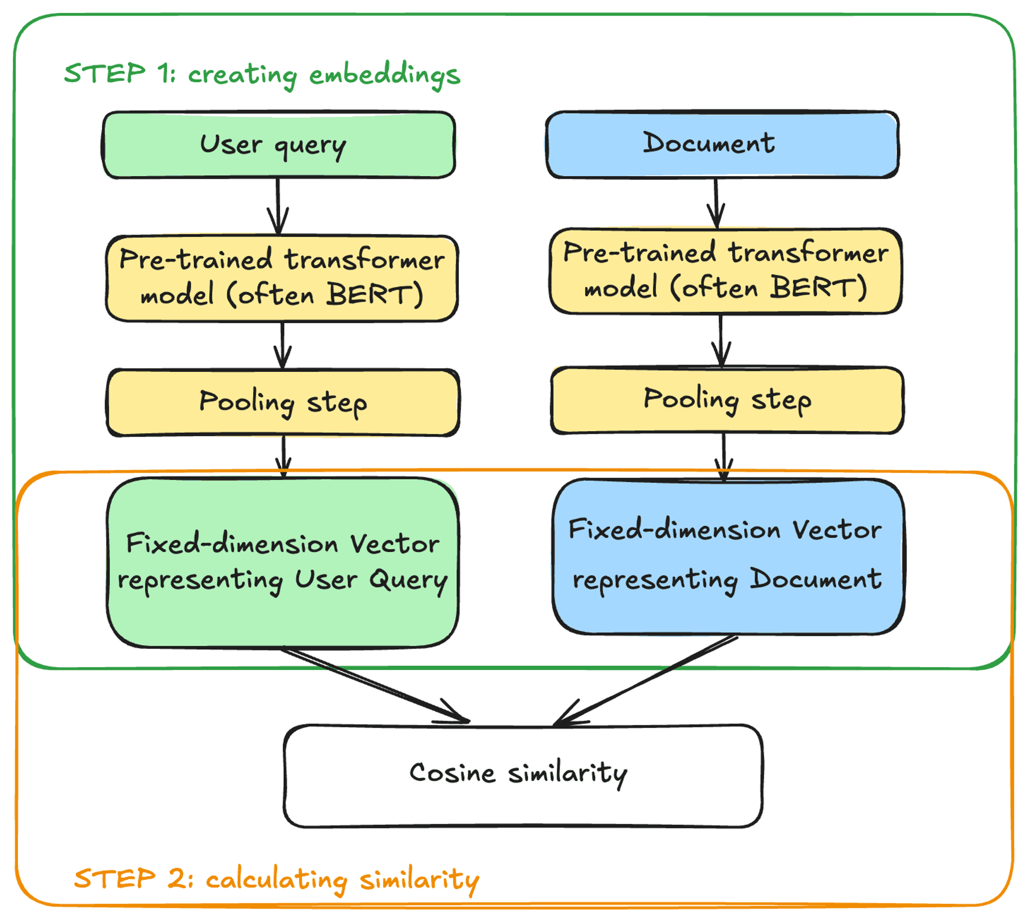
In this setup, document and query vector representations are computed using the same embedding model, but in complete isolation from each other. The model never sees the documents and user queries simultaneously. This is important because it enables us to generate document embeddings at any point in time and store them in a vector store. At inference time, only the user query embedding needs to be computed to run the similarity search and find documents with similar vector representations.

What about Cross-Encoder embedding models? How do they work? A Cross-Encoder takes in both text pieces (e.g. a user query and a document) simultaneously. It does not produce a vector representation for each of them, but instead outputs a value between 0 and 1 indicating the similarity of the input pair. 

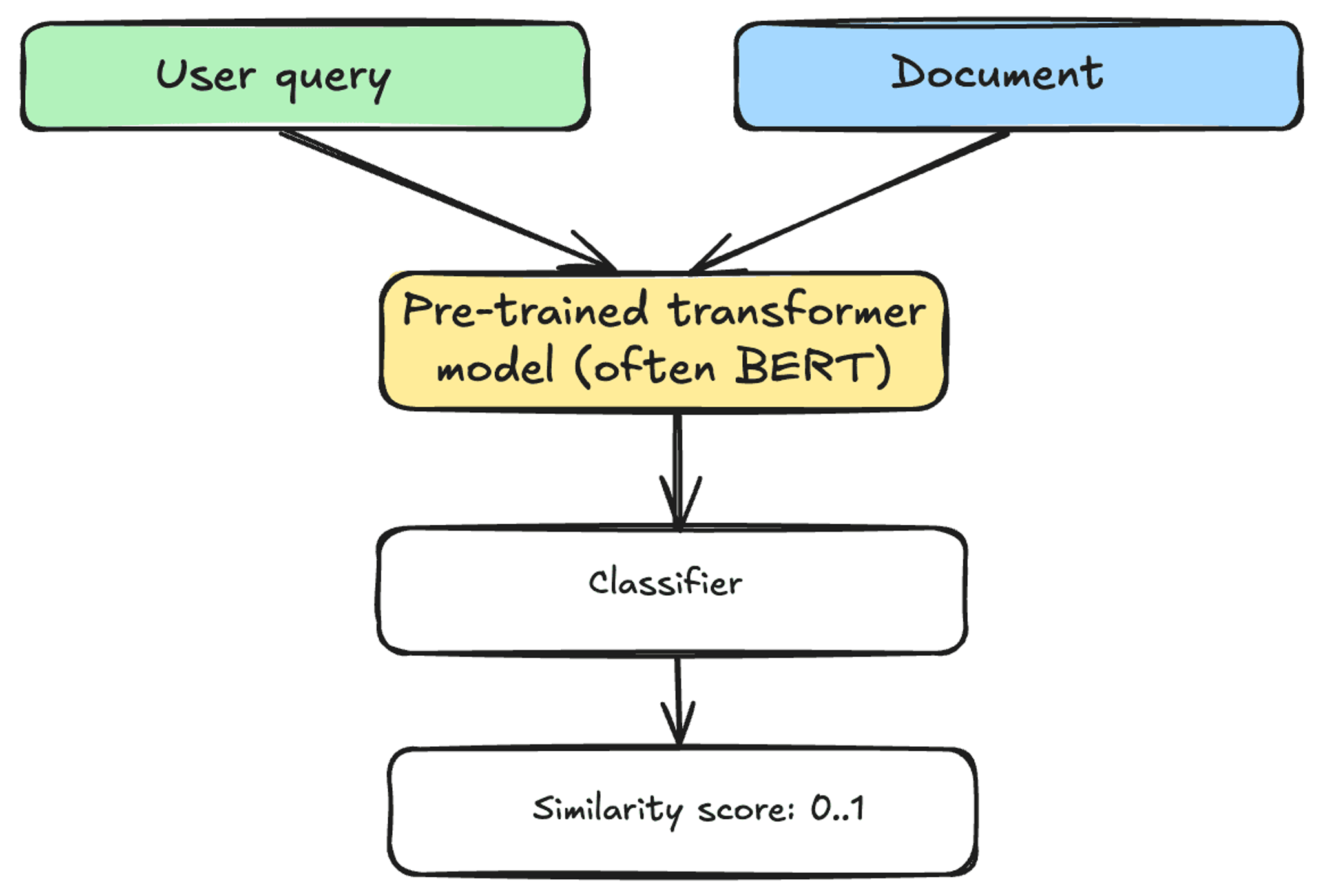
Because Cross-Encoders have access to both user query and the document at the same time, they have shown to achieve better performances at identifying similar documents compared to Bi-Encoders. However, this comes at the cost of computational efficiency. With Bi-Encoders, you can pre-compute embeddings for millions of documents ahead of time and leverage fast Approximate Nearest Neighbors (ANN) algorithms provided by vector stores to find similar vector representations.

In contrast, Cross-Encoders would require calculating scores for each query and each of the millions of documents, which is not feasible at inference time. Nevertheless, their strength in capturing nuanced relationships between the query and candidate documents makes them an excellent choice as a reranker. Once you've retrieved a batch of candidates, you’re working with a small set of documents, and you can use a reranker to re-assess the similarity to the original query. Using a Cross-Encoder at this stage is computationally manageable and allows you to leverage its strengths and improve the accuracy of the retrieval.

For the initial embedding of documents, however, a Bi-Encoder is necessary. Let's take a closer look at how these models are trained and benchmarked to understand how to select the best one for your specific use case.

How Bi-Encoder models are pre-trained and benchmarked

Pre-training an embedding model

Although training steps may vary slightly from one model to another, and not all model publishers have shared their training details, the pre-training steps for Bi-Encoder embedding models generally follow a similar pattern.

The process begins with a pre-trained general-purpose encoder-style model, such as a small, ~100M-parameter pre-trained BERT. Despite the availability of larger, more advanced generative LLMs, this smaller BERT model remains a solid backbone for text embedding models today.

To fine-tune the pre-trained BERT for information retrieval, a dataset is assembled consisting of text pairs (question/answer, query/document) with a contrastive learning objective that reflects the downstream use of text embeddings. The text pairs can be positive (e.g. a question and an answer to it), and negative (a question and unrelated text). The goal is for the model to learn to bring the embeddings of positive pairs closer together in vector space while pushing the embeddings of negative pairs apart. 

The training process often has more than one step. Initially, the model is trained on a large corpus of text pairs in a weakly supervised manner. However, to achieve SOTA results on the leaderboards, a second round of contrastive training is often employed. In this second round, the model is further trained on a smaller dataset with high-quality data and particularly challenging examples from academic datasets like MSMARCO, HotpotQA, and NQ. This training recipe delivers strong general-purpose embedding models that top the MTEB leaderboard. Given the importance of the MTEB leaderboard in guiding the choice of embedding model, let's take a closer look at what the MTEB benchmark is.

Embedding model benchmarks

Evaluating the quality of embedding models within retrieval systems in general, and not within a context of a specific use case, can be challenging. Decades of academic research have led to the development of the Massive Text Embedding Benchmark (MTEB) that has become a standard benchmark for text embedding models.

MTEB spans 8 embedding tasks, including bitext mining, classification, clustering, pair classification, reranking, retrieval, STS (semantic textual similarity), and summarization. At the time of writing, it covers a total of 181 datasets spanning multiple domains, text lengths, and languages. This is the most comprehensive public benchmark of text embeddings to date. For the purpose of evaluating embedding models for RAG, we focus on the Retrieval tab of the MTEB leaderboard.

A widely used metric for evaluating a model’s retrieval performance is Normalized Discounted Cumulative Gain @ 10 (NDCG@10). There are other metrics, of course, such as Precision@K, Recall@K, and more, but NDCG is a standard benchmarking metric that assesses the quality of an ordered list of results or predictions. NDCG@10 specifically evaluates the top 10 retrieval results. The calculation of NDCG considers both the relevance of each result and its position in the list. The metric ranges from 0 to 1, where 1 indicates a perfect match with the ideal order, and lower values represent a lower quality of the results ranking. In the leaderboard, you can find out how well different embeddings model perform at information retrieval (measured with NDCG@10) under the Retrieval tab. 

You can check the average scores across for the embedding models, but depending on your specific RAG application you may also want to refine your selection. For instance you may want to narrow down your choices to a specific language (e.g., English, Chinese, French, Polish) or domain (e.g., law). 

Even within a language, there’s room for nuance. We won’t cover all of the datasets here, but let’s take a brief look at the datasets used to measure retrieval performance for embedding models in English language:

• ArguAna: pairs of arguments and counterarguments scraped from an online debate portal. 

• ClimateFEVER: dataset for verification of climate change-related claims

• CQADupstackRetrieval: community question-answering dataset with data from 12 different StackExchange subforums: Android, English, Gaming, Gis, Mathematica, Physics, Programmers, Stats, Tex, Unix, Webmasters and Wordpress.

• DBPedia: a set of heterogeneous entity-bearing queries containing named entities, IR style keywords, and natural language queries.

• FEVER: a dataset build for fact verification systems on real-world misinformation

• FiQA2018: opinion based question-answer pairs for financial data by crawling StackExchange posts under the Investment topic from 2009-2017 as our corpus

• HotpotQA: multi-hop questions which require reasoning over multiple paragraphs to find the correct answer. Answers source - Wikipedia.

• MSMARCO

• NFCorpus: contains natural language queries harvested from NutritionFacts and annotated medical documents from PubMed

• NQ: Google search queries and documents with paragraphs and answer spans within Wikipedia articles.

• QuoraRetrieval:

• SCIDOCS: scientific papers and direct-citations

• SciFact: a dataset for fact checking scientific claims

• Touche2020: a conversational arguments dataset

• TRECCOVID: biomedical. Queries and scientific articles related to the COVID-19 pandemic

A model with the highest average score across all of these dataset will give you a well rounded general purpose model, but if your data is mostly financial, for example, you may care more about the NDCG@10 score on the FiQA2018 dataset than, say, TRECCOVID, or ClimateFever. 

Choosing your baseline embedding model

Now that you know how embedding models work, how they are trained and how they are academically benchmarked, let’s list the practical tips for choosing an appropriate embedding model: 

• Look for a bi-encoder on the MTEB Leaderboard. For a RAG application, check out the “Retrieval” task, and explore the NDCG@10 score for datasets in your language and domain. A higher NDCG@10 score indicated a better performance.

• Start with a small embedding model. First, the model size directly impacts latency. Second, a smaller model will let you build a quick baseline upon which you can iterate. Finally, a larger model is not necessarily better for your particular use case. It may be overfit on the training data and academic datasets to score high on the leaderboard but it may not translate into the best performance on your custom data. 

• Choose an embedding model with a reasonably-sized max tokens for your case. The max tokens value indicates the maximum size of document chunks you can embed with the model. In most cases, you won’t need to embed large documents as a whole, in fact for precise retrieval, smaller chunks are typically preferable. Learn about the importance of chunk sizes in our recent blog post. 

• Finally, don’t forget to check the license of the embedding model of your choice, so that you are allowed to use it commercially, if that is your intent. 

Once you have selected your embedding model, you can easily add it to your data preprocessing pipeline with Unstructured with only a couple of lines of code: 

embedder_config=EmbedderConfig(
   embedding_provider="langchain-huggingface",
   embedding_model_name=os.getenv("EMBEDDING_MODEL_NAME"),
),

Even though in this blog post we have used Hugging Face Leaderboard as an example for comparing embedding models, it doesn’t mean that a model in your unstructured data ETL necessarily has to come from the Hugging Face Hub. 

In fact, Unstructured supports multiple embedding model providers, and you can choose whichever you prefer: OpenAI, HuggingFace, AWS Bedrock, Vertexai, Voyageai, or OctoAI.

You can learn more about embedding configuration with Unstructured in our documentation, and find ETL examples in our notebook collection. 

Once you have your embedding model pick, don’t rely solely on the MTEB benchmark! Evaluate the embedding model on a subset of your own data .

Improving the retrieval performance

Selecting an appropriate baseline embedding model and integrating it into your preprocessing pipeline is the great first step. From then on you can always continue optimizing the retrieval performance of your RAG system. Here are some of the knobs you can turn:

• Optimize chunk sizes. While smaller chunks generally enhance precision, there is no one-size-fits-all approach. Experiment with different chunk sizes to find the sweet spot for your use case. Learn more about chunking best practices. 

• Hybrid search. If your data contains acronyms, domain-specific words, product names or codes that the embedding model was never exposed to, adding keyword search in addition to similarity search will improve retrieval in this situation without adding computational overhead. 

• Utilize metadata. Documents do not exist in isolation. For every document type Unstructured extracts metadata that you can use to filter the results. 

• Add a reranker step: as mentioned earlier, cross-encoders take in both a user query and a document and are better than bi-encoder combined with similarity search at identifying related pairs. They are inefficient to run over the whole knowledge base, but they can improve the results, if you first retrieve documents with hybrid search, and then apply a cross-encoder as a reranker. 

• Fine-tune the embedding model. One of the things that you can do to improve the retrieval performance of your RAG system is fine-tuning your embedding model on your data to teach it to match the unique types of questions your users ask to document pieces they expect to have answers. To do so, you won’t need millions of real-world user query examples to start the fine-tuning experiments, you may be able to get by with just a few thousand. 

Conclusion

Selecting the right baseline embedding model for a RAG system can be a daunting task, but with the right tools and knowledge, it can be made much easier. By understanding the differences between Bi-Encoders and Cross-Encoders, and how they are trained and evaluated, you can make informed decisions about which model to use for your specific use case. 

The Massive Text Embedding Benchmark (MTEB) leaderboard provides a valuable resource for evaluating the performance of different embedding models, and by considering factors such as language, domain, and task-specific performance, you can refine your selection to find the best model for your needs. 

Once you choose the right embedding model, you can integrate it into your Unstructured ETL pipeline with just a few lines of code, no matter where your embedding model is hosted. 

Get your Serverless API key today and build your RAG with confidence! We cannot wait to see what you build with Unstructured Serverless. If you have any questions, we’d love to hear from you! Please feel free to reach out to our team at hello@unstructured.io or join our  Slack community.